Generating Fractals by Finding Roots With Halley's Method

December 10, 2025

The results for finding the roots for the function f(z) = z^3 - 1 aren’t super impressive. That’s what is shown in the “Basins of attraction” image on the left:

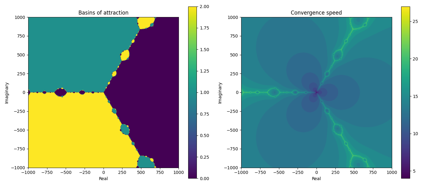
The “Convergence speed” image on the right is more interesting, but the key to the math seems to be related to what’s happening in the simpler image.

Basins of attractors

Here’s a scaled down version of the complex plane that’s used to generate the image:

In [9]: x = np.linspace(0, 4, 5)

In [10]: y = np.linspace(0, 4, 5)

In [11]: X, Y = np.meshgrid(x, y)

In [12]: Z = X + 1j * Y

In [13]: Z
Out[13]:
array([[0.+0.j, 1.+0.j, 2.+0.j, 3.+0.j, 4.+0.j],
       [0.+1.j, 1.+1.j, 2.+1.j, 3.+1.j, 4.+1.j],
       [0.+2.j, 1.+2.j, 2.+2.j, 3.+2.j, 4.+2.j],
       [0.+3.j, 1.+3.j, 2.+3.j, 3.+3.j, 4.+3.j],
       [0.+4.j, 1.+4.j, 2.+4.j, 3.+4.j, 4.+4.j]])

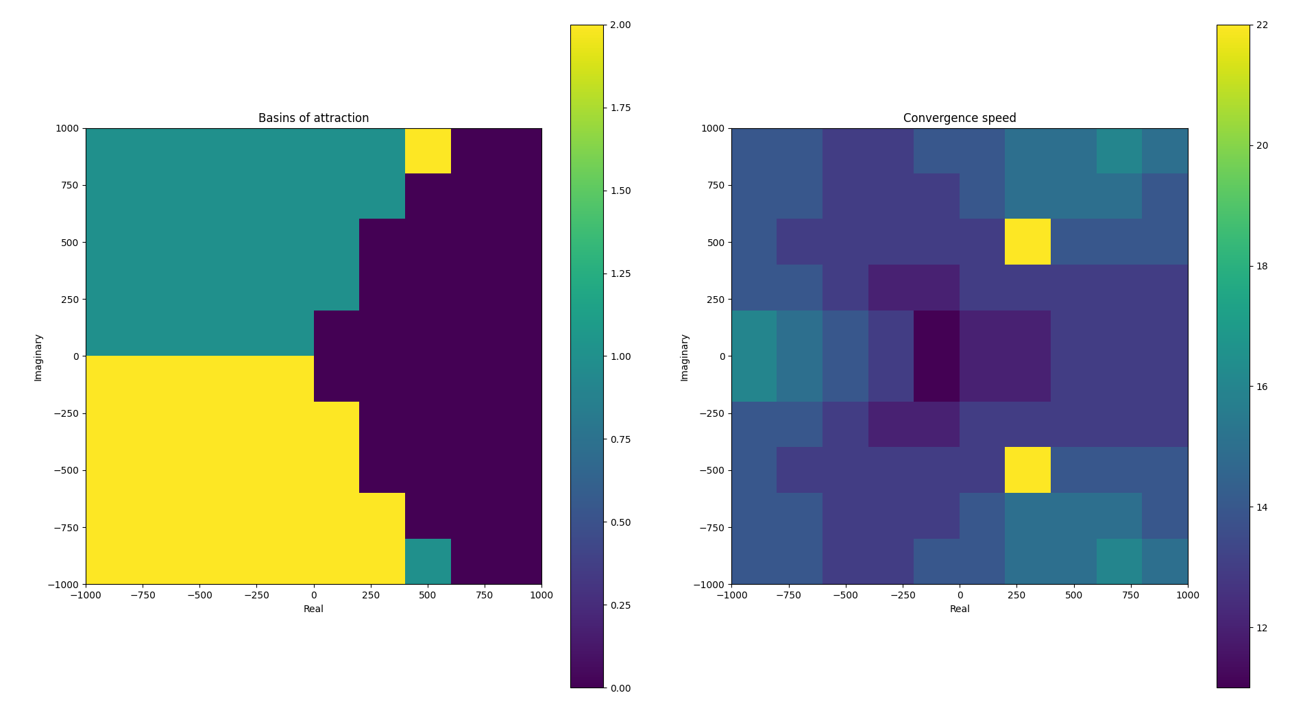
Z is a (5, 5) complex plane. Scaling things up a tiny bit, here’s the result of running the halleys_root_fractal function function with a (10, 10) complex plane, and the function f(z) = z^3 - 1:

For any starting point z_0 in the complex plane, Halley’s method generates a sequence:

z_{n+1} = z_n - (2f(z_n)f'(z_n))/(2f'(z_n)^2 - f(z_n)f''(z_n))

It might be clearer to look at a code implementation:

fz = f(z)
dfz = df(z)
ddfz = ddf(z)
denominator = 2 * dfz**2 - fz * ddfz
z = z - (2 * fz * dfz) / denominator  # update the z variable

The following code generates 12 initial z0 coordinates. The coordinates are each separated by 30 degrees (2 * np.pi / 12) around a circle with a radius of 1.5:

angles = np.linspace(0, 2 * np.pi, 12, endpoint=False)
radius = 1.5

for angle in angles:
    z0 = radius * np.exp(1j * angle)

The list of 12 z0 values:

z0.real: 1.5000, z0.imaginary: 0.0000
z0.real: 1.2990, z0.imaginary: 0.7500
z0.real: 0.7500, z0.imaginary: 1.2990
z0.real: 0.0000, z0.imaginary: 1.5000
z0.real: -0.7500, z0.imaginary: 1.2990
z0.real: -1.2990, z0.imaginary: 0.7500
z0.real: -1.5000, z0.imaginary: 0.0000
z0.real: -1.2990, z0.imaginary: -0.7500
z0.real: -0.7500, z0.imaginary: -1.2990
z0.real: -0.0000, z0.imaginary: -1.5000
z0.real: 0.7500, z0.imaginary: -1.2990
z0.real: 1.2990, z0.imaginary: -0.7500

Given the following function f and its derivatives:

# f(z) = z^3 - 0.1
def f(z):
    return z**3 - 0.1


def df(z):
    return 3 * z**2


def ddf(z):
    return 6 * z

The three roots of the function (broken down to real and imaginary parts) are:

real: 0.4641588833612779, imaginary: 0.0
real: -0.23207944168063885, imaginary: 0.4019733843830849
real: -0.23207944168063915, imaginary: -0.4019733843830847

Tracing the path of a single z0 point

Passing the first z0 value (z0.real: 1.5000, z0.imaginary: 0.0000) through Halley’s method until it converges generates the following real and imaginary parts:

z.real: 0.7828467153284673, z.imag: 0.0
z.real: 0.502252315722975, z.imag: 0.0
z.real: 0.4643100491277034, z.imag: 0.0
z.real: 0.46415888337196165, z.imag: 0.0

It converges in a straight line to z.real: 0.46415888337196165, z.imag: 0.0, that’s approximately the root (real: 0.4641588833612779, imaginary: 0.0). The code stops the convergence process at that point.

Here’s a plot of the paths taken by all 12 points listed above:

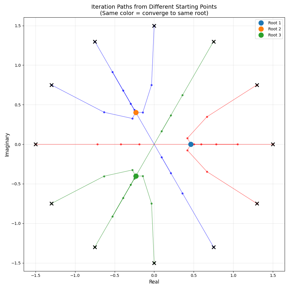
code used for generating this image

The first z0 point (z0.real: 1.5000, z0.imaginary: 0.0000) is the “X” symbol at point (1.5, 0). The small red dots show it converging towards the root real: 0.4641588833612779, imaginary: 0.0 (the blue dot).

Iterations of Halley’s method preserve symmetry

What’s interesting in the plot is the paths taken by the 3rd, 7th, and 11th z0 values. These starting points are special because they lie exactly on the boundaries between basins of attraction (they are on angular bisectors(?)):

3rd point: angle 60 degrees (between roots 0 degrees and 120 degrees)
7th point: angle 180 degrees (between roots 120 and 240 degrees)
11th point: angle 300 degrees (between roots 240 and 360/0 degrees)

Halley iterations (and Newton method iterations (?)) preserve symmetry. If a point starts at an angle that’s equidistant from two roots, the iteration keeps it on that line.

Intuitively, it seems that there’s be no way for it to know where to go — it’s being “pulled” equally from the equidistant roots. But what’s doing the pulling?

The hesitation effect

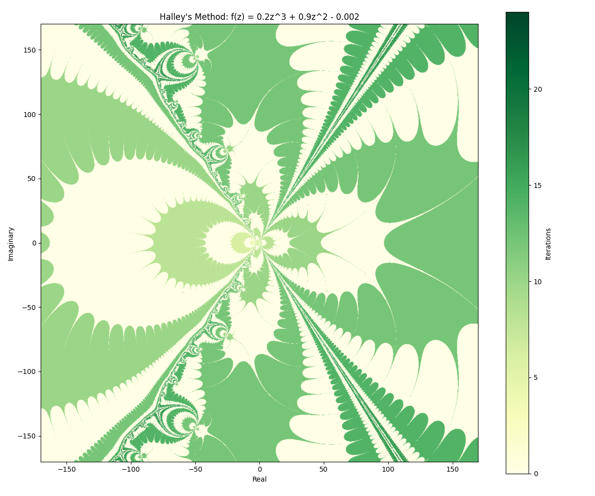
I’ll post the image from the top of this note again here:

It demonstrates how the symmetry lines between the basins of attraction relate to convergence speed. The yellow patterns along the symmetry lines indicate that it took more iterations for points in a region to converge on a root. I need to confirm this, but it seems to indicate that points near symmetry lines are (somehow) “pulled” towards adjacent roots. This results in slow “decision making”, and delayed convergence.

The suggestion (from Claude) is that numerical error eventually pushes it towards a boundary. Possibly it’s something else: Notes on Cognitive and Morphological Patterns.

Tags:

Math