Halley's root finding code analysis
Related to Generating fractals with Halley’s Method . The Halley’s Method note has an overview of the math.
The full code is at Halley’s which-root code.
An attempt to look at what’s going on with the math: notes / Generating fractals by finding roots with Halley’s Method.
Generate fractals by checking for convergence on known roots #
Starting with the (poorly named) halleys_roots_fractal function.
Create a grid of complex numbers #
def halleys_roots_fractal(
    f,
    df,
    ddf,
    roots,
    width=800,
    height=800,
    xmin=-2.0,
    xmax=2.0,
    ymin=-2.0,
    ymax=2.0,
    max_iter=50,
):
    # create a grid of complex numbers
    x = np.linspace(xmin, xmax, width)
    y = np.linspace(ymin, ymax, height)
    X, Y = np.meshgrid(x, y)
    Z = X + 1j * Y
    # ...
A simplified demonstration of np.meshgrid:
In [28]: x = np.array([0, 1, 2, 3, 4])

In [29]: y = np.array([0, 1, 2, 3, 4])

In [30]: X, Y = np.meshgrid(x, y)

In [31]: X
Out[31]:
array([[0, 1, 2, 3, 4],
       [0, 1, 2, 3, 4],
       [0, 1, 2, 3, 4],
       [0, 1, 2, 3, 4],
       [0, 1, 2, 3, 4]])

In [32]: Y
Out[32]:
array([[0, 0, 0, 0, 0],
       [1, 1, 1, 1, 1],
       [2, 2, 2, 2, 2],
       [3, 3, 3, 3, 3],
       [4, 4, 4, 4, 4]])
Starting with the 1D arrays, x and y, meshgrid creates 2 2D arrays where every possible
combination of the x and y coordinates exists. meshgrid returns a tuple: (X, Y). When it’s
called with X, Y = np.meshgrid(x, y), the tuple is being unpacked into the X and Y variables.
In the fractal function code, the ranges defined by x and y are used to generate a grid (2 2D
arrays). The Z array is a 2D matrix of complex numbers (in the rectangular form) where the real
part is set from X and the imaginary part is scaled by Y.
Create matrices to store the output #
The function is going to run Halley’s Method against every point in the Z matrix and record what
root the point converges on, and how many iterations it takes to converge.
    # ...
    # record the index of the root that a point converges on
    # the index used is the index from the `roots` function argument
    root_map = np.zeros((height, width), dtype=int)
    # record how many iterations it takes for a point to converge
    iter_map = np.zeros((height, width), dtype=int)
    # ...
Iterate through the grid of complex numbers #
    # ...
    for i in range(height):
        for j in range(width):
            z = Z[i, j]  # the complex number
      # ...
Call Halley’s Method on a point #
            # ...
            for iteration in range(max_iter):
                fz = f(z)
                dfz = df(z)
                ddfz = ddf(z)

                if abs(fz) < 1e-6:  # considered to be converged if magnitude < 1e-6
                    distances = [abs(z - root) for root in roots]
                    root_idx = np.argmin(distances)
                    root_map[i, j] = root_idx
                    iter_map[i, j] = iteration
                    break

                denominator = 2 * dfz**2 - fz * ddfz
                # avoid divide by zero errors; hasn't been called yet when testing
                if abs(denominator) < 1e-15:
                    print("Denominator approaching zero; breaking from loop")
                    break
                z = z - (2 * fz * dfz) / denominator
                # ...
fz = f(z): f is the function that roots are being found for. E.g.:
# f(z) = z^3 - 1
def f(z):
    return z**3 - 1
df is the function that calculates the first order derivative. E.g.:
def df(z):
    return 3 * z**2
ddf is the function that calculates the second order derivative. E.g.:
def ddf(z):
    return 6 * z
Refer to notes / Halley’s Method for details about how Halley’s Method works (note that I don’t provide a proof of it there). What’s significant for this implementation is:
                if abs(fz) < 1e-6:  # considered to be converged if magnitude < 1e-6
                    distances = [abs(z - root) for root in roots]
                    root_idx = np.argmin(distances)
                    root_map[i, j] = root_idx
                    iter_map[i, j] = iteration
                    break
When abs is called on a complex number, it returns the magnitude of the number — the part
(radius) of the exponential form of the number. When the radius is less than 1e-6, the function
considers it to be converged.
It then finds the root (from the roots array argument) that the value of z that the fz
function was called with that’s closest to:
distances = [abs(z - root) for root in roots]
root_idx = np.argmin(distances)
The root index for the current point is saved to root_map[i, j]. The number of iterations of
Halley’s Method that it took to converge to the root is saved to iter_map[i, j].
That’s basically it. The rest of the function just handles the case of a point that’s failed to
converge, and returns the values that are needed to render the root_map and iter_map as images:
            # ...
            else:  # for...else is legitimate Python; runs if a break statement isn't hit in the for loop
                # didn't converge
                root_map[i, j] = -1
                iter_map[i, j] = max_iter

    return root_map, iter_map, x, y
Supplying the function arguments #
def halleys_roots_fractal(
    f,
    df,
    ddf,
    roots,
    width=800,
    height=800,
    xmin=-2.0,
    xmax=2.0,
    ymin=-2.0,
    ymax=2.0,
    max_iter=50,
):
f, df, and ddf are functions. E.g.:
# f(z) = z^3 - 1
# the function to find the roots for
def f(z):
    return z**3 - 1

# the first order derivative
# e.g.: if f(x) = x^5; f'(x) = 5x^(5-1)
def df(z):
    return 3 * z**2

# the second order derivative
# e.g.: if f(x) = 3x^2; f'(x) = 3*2x^(2-1)
def ddf(z):
    return 6 * z
Finding the roots of function f #
The need to find the roots is the annoying part of this implementation. Annoying in the sense that
it makes it difficult to just quickly test a bunch of functions. The roots for f(z) = z^3 - 1 are:
roots = [1, np.exp(2j * np.pi / 3), np.exp(4j * np.pi / 3)]
Go to the Roots of f(x) = x^3 -1 section for more details, or have a look at these links:
Setting the size and coordinates of the complex plane #
The xmin, xmax, ymin, and ymax arguments set the size and position of the complex plane that
Halley’s Method is run against. E.g., xmin=-1000, xmax=1000, ymin=-1000, ymax=1000 will generate a
plane with the real (x) axis in the range (-1000, 1000) and the imaginary (y) axis in the range
(-1000, 1000). The center of the plane will be the point (0, 0).
The height and width arguments set the actual number of points that will exist in the range set
by the xmin/xmax, ymin/ymax arguments.
Calling the function and rendering images with PyPlot #
# f(z) = z^3 - 1
def f(z):
return z**3 - 1
def df(z):
return 3 * z**2
def ddf(z):
return 6 * z
roots = [1, np.exp(2j * np.pi / 3), np.exp(4j * np.pi / 3)]
root_map, iter_map, xs, ys = halleys_roots_fractal(
af,
df,
ddf,
alt_roots,
xmin=-1000,
xmax=1000,
ymin=-1000,
ymax=1000,
)
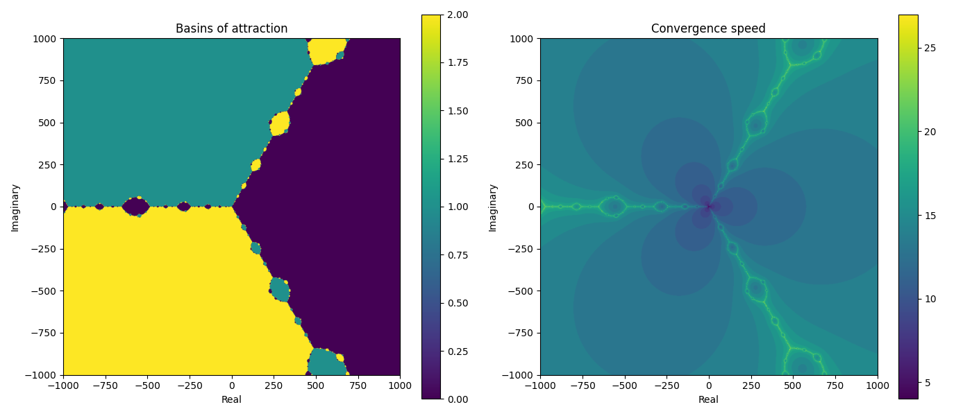
fig, (ax1, ax2) = plt.subplots(1, 2, figsize=(14, 6))
# map which roots are selected for the complex points
im1 = ax1.imshow(
root_map, extent=(xs[0], xs[-1], ys[0], ys[-1]), cmap="viridis", origin="lower"
)
ax1.set_title("Basins of attraction")
ax1.set_xlabel("Real")
ax1.set_ylabel("Imaginary")
cbar1 = plt.colorbar(im1) # could use cbar1.set_label("some label") to set a label
# map how many iterations it took each point to converge on its root
im2 = ax2.imshow(
iter_map, extent=(xs[0], xs[-1], ys[0], ys[-1]), cmap="viridis", origin="lower"
)
ax2.set_title("Convergence speed")
ax2.set_xlabel("Real")
ax2.set_ylabel("Imaginary")
cbar2 = plt.colorbar(im2)
plt.tight_layout()
plt.show()
The full source code is at Halley’s Which Root Code
Roots of f(x) = x^3 - 1 #
Starting with the function f(x) = x^3 - 1. The roots will be x^3 = 1
First guess: There’s a real root of 1: 1 * 1 * 1 = 1, that is also the complex number 1 + 0i.
Systematic approach:
Express 1 in the exponential form
- r (magnitude):
1 - \theta (angle from the positive real axis):
So 1 can be written in the exponential form as , or more simply as
But the trick is that is the same as , because has a period of . So:
In general, for any integer .
What actually gets solved for is:
By convention, use to generate distinct roots. For the cubic roots, .
In the code below, the 1 root comes from k=0; e^0 = 1; the np.exp(2j * np.pi/3 comes from k=1 (the 2 in 2j comes from 1*2); in the last root, the 4 in 4j comes from k=2; 2*2=4:
roots = [1, np.exp(2j * np.pi / 3), np.exp(4j * np.pi / 3)]
Roots of f(x) = x^3 - 0.1 #
See Solving polynomial equations
roots = [0.1**(1.0/3), 0.1**(1.0/3) * np.exp(2j * np.pi / 3), 0.1**(1.0/3) * np.exp(2j * np.pi / 3)]