Real and complex numbers in space

Real numbers ($R$) are numbers that can be found on a number line. What’s a number line?

Understanding dimensions

The physical world is normally understood to have three dimensions. A sheet of paper is conceptually a two dimensional object (ignoring its thickness). A one dimensional object (with similar relaxed constraints) could be a piece of string or wire, a timeline,…, essentially any continuous variable plotted on an axis.

The dimensionality of an object can maybe be considered as the degrees of freedom that the object has. A number line can be considered to be a 2D object. It’s constrained to $-\inf \leftarrow, \dots, \inf$.

In the physical world, all objects are going to be projected onto three dimensions — 1D, 2D, 4D, etc, are largely conceptual.

Complex numbers have an extra dimension

Complex numbers have an extra dimension: $i = \sqrt{-1}$.

Visualizing complex numbers

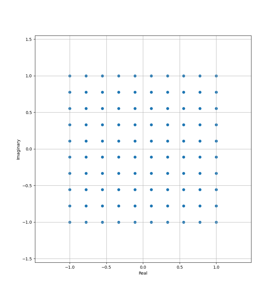
Complex numbers can be visualized on a 2D plane. The following code creates a 10x10 grid of complex numbers, with the real plane in the range (-1, 1) and the real part of the complex plane also in the range (-1, 1):

import numpy as np
import matplotlib.pyplot as plt

xmin = -1.0
xmax = 1.0
ymin = -1.0
ymax = 1.0
width = 10
height = 10


x = np.linspace(xmin, xmax, width)
y = np.linspace(ymin, ymax, height)
X, Y = np.meshgrid(x, y)
Z = X + 1j * Y

# Scatter plot the points on the complex plane
plt.scatter(Z.real, Z.imag)
plt.xlabel("Real")
plt.ylabel("Imaginary")
plt.axis("equal")
plt.grid(True)
plt.show()

Complex numbers can be visualized as vectors.

# A quiver plot is a 2D graph that displays a field of vectors as arrows.
# quiver([X, Y], U, V, [C], /, **kwargs)
# X, Y define the arrow locations, U, V define the arrow directions.
# The `angles` arg sets the direction of the arrows; "xy": arrows point from (x, y) to
# (x+u, y+v)
plt.quiver(
    Z.real,  # arrow X coordinate start
    Z.imag,  # arrow Y coordinage start; the r part of the imaginary number
    Z.real,  # point arrows in the direction of the complex number
    Z.imag,  # point arrows in the direction of the complex number
    angles="xy",
    scale_units="xy",
    scale=1,
)

Here’s a scaled down version of the complex numbers that are being used in these examples. It’s a 4x4 grid instead of a 10x10 grid:

 [[-1.        -1.j         -0.33333333-1.j          0.33333333-1.j        1.        -1.j        ]
 [-1.        -0.33333333j -0.33333333-0.33333333j  0.33333333-0.33333333j 1.        -0.33333333j]
 [-1.        +0.33333333j -0.33333333+0.33333333j  0.33333333+0.33333333j 1.        +0.33333333j]
 [-1.        +1.j         -0.33333333+1.j          0.33333333+1.j         1.        +1.j        ]]

Calculating the angle for a complex number (also called the argument or phase)

Starting from a complex number in the rectangular form: -0.33333333-1.j

Identify the components:

• real part: -0.33333333
• imaginary part: -1.0

The number is a + bi = -0.33333333-1j

Visualize (imagine for now) the number on the complex plane:

x = -0.33333333, y = -1.0. The number is in the third quadrant, both x and y are negative.

Calculate the angle of the point:

The simple approach with Python is theta = np.arctan2(y, x), or theta = np.angle(-0.33333333-1j)

In [10]: np.angle(-0.33333333-1j)  #   np.float64(-1.8925468781915389)
Out[10]: np.arctan2(-1, 0.33333333)  # np.float64(-1.8925468781915389)

Note that np.angle returns the angle of a complex number in radians, np.arctan2 returns the angle of (opposite, adjacent), (x, y), (real, imag).

Related

• notes / Solving polynomial equations > solving polynomial equations for complex roots